Excel makes work easier for its users, but some shortcuts, formulas, and tips will make the work even easier once the user becomes familiar with working with them. Below, I will take you through some of these tips that will make your work easier.
Formulas
. Excel formulas help identify the relationship between cells of a spreadsheet, perform mathematical calculations of those values, and return the results to the cells of your choice. Formulas one can automatically apply include array, count, average, trim, sum, if, and date.
1. Array. This formula is used to calculate and return values of multiple ranges rather than a single cell added or multiplied together.
formula = {(start value 1; end value 1) *(start value 2: end value 2)}
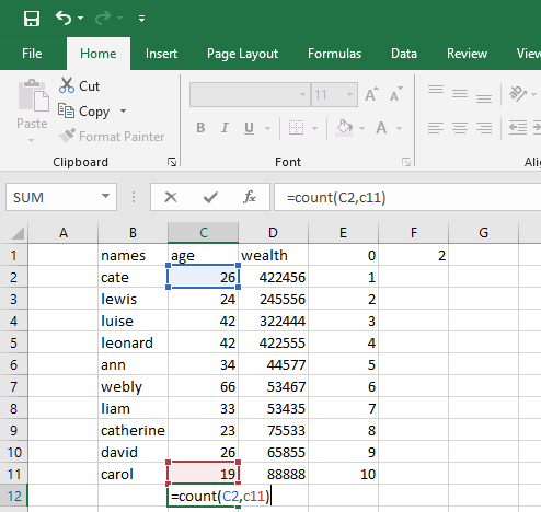
2. Count. This is a formula used to get the number of entries of a number field in a range or array of numbers. It only works on numeric values, unlike count, which calculates all the data in cells despite their nature.
Formular= count (start value 1, End value 1)
3. Trim. It is a formula used to remove any space before and after a text in an excel worksheet cell.
Formular=Trim(text)
Trim only works on a single cell, unlike other functions that can work in a range of selected cells and hence the downside of adding duplicate data on the spreadsheet. An example is as shown below

4. Sum. It gives the total values from a selected range, be it in the columns or the rows, respectively.
5.
Date/time
Excel date formula returns a date that corresponds to the value entered in the parentheses and even other values from other cells.
= Date (year, month, and day)
This can be seen as a handy task, but the two methods can execute it.
Creating dates from a series of cell values. Select an empty cell and type = dates in the formula bar and enter the cells whose value create your desired date
Automatically select today's date.to do this, follow the following step. = DATE (YEAR(TODAY ()) MONTH(TODAY())DAY(TODAY()) then press enter, and it will return the current date on the working of your worksheet.
6. Average. A formula of excel which calculates an average of numbers or values from a selected range.
Formula= Average (start value1, end value 1)
Example. Calculation of average wealth in column D = average(D2, D11) as shown below

7. IF.it is used when working on sorting data according to a given logic, and one can embed the function and the formula in it.
=if{(logical_test_true) (logical_test_false)}
Keyboard shortcuts
Shortcuts are an overlooked way of improving productivity in excel works. The use of keys instead of typing or scrolling through the toolbar improves efficiency and speed drastically. Below are some of the excel shortcuts one should know when and where to apply while working in a spreadsheet to help save on time.
1. Add a border to cells
The keyboard shortcut for adding an outer border to the selected cell is
Alt+H, B
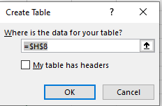
2. Insert table
PC: ctrl T
After you use this command, a pop-up menu will show up on the screen asking where you want to insert your table.
3. Select the entire row.
Pc: Shift + space
A single press on this command key row will be selected. If you want to select multiple rows, hold the shift key and the up and down arrow to move to the rows you want to select.
4. Select the entire column
PC: Ctrl + space
This can be a great time-saver, like in the use of command keys to select the rows. Tip, hold on the shift key and use the right/left arrow to move across, selecting multiple columns.
5. Hide rows in a worksheet
PC; ctrl + 9
If you do not want sensitive data in some rows to be visible in your worksheet, it is possible to hide those rows. The use of the above command keys makes the work easier and saves you a lot of time. You can also use the hide rows to avoid printing them while making a hard copy.
6. Copy formula from the above cell.
Pc: Ctrl + '
This is an easy and time-saving way of applying a formula from one cell to the one down next to it and keeping the cell reference.
7. Copy value from the cell above.
Ctrl + shift+ "
This is the formula you apply to copy the value in an above cell without copying the formula used in that reference cell.
Tricks applicable in excel that will save you time
These are smart instructions and guides on applying functions and formulas to make work easy to excel. Below are some of the tips applicable in excel.
1. Insert function.
This is an easy way of inserting a formula from the ribbon of the worksheet. You go to the formula tab and click on the insert function and choose the formula needed. As shown below.

2. Remove duplicate data on excel
Select the range of cells that have duplicate values you want to remove. Click data, remove duplicates, and then under columns, check or uncheck the columns where you want to remove the duplicates and click ok.
3. Slip up text information between columns
You can take the text and slip up the information in more than one cell into multiple cells using the converter wizard.
Steps.
Select the cell or the column that contains the information you want to slip, select the data, text to columns, convert the text to columns wizard, select delimited, next, and select the delimiter for your data.
4. Hyperlinking a cell to a website.
On the worksheet, click on the cell which you want to create a hyperlink; on the insert tab, click hyperlink; under the display checkbox, type the text that you want to use to represent the hyperlink, then under the URL, type the complete URL of the webpage you want to link.
5. Deleting blank cells.
The best way to delete blank cells and maintain accuracy when calculating the mean and sum in an excel sheet is by filtering the blank cells and deleting them. You go Data>filter>select all then choose the last optional the blanks, all the blank cells will show, go back home, and press delete and all the blanks cells will be deleted.
6. Input restriction with data validation
You go to Data, data validation>settings, input the condition, and shift to input message to give promptly. The user will get this prompt when hanging the pointer in this area and get a warning message if the inputted information is unqualified.
7. Use COUNTIF function to make excel count words or numbers in any range of the cell
COUNTIF function is used for counting cells within a specified range that meet a certain criterion or condition. For example, you can write a COUNTIF formula to determine how many cells in your worksheet contain a number greater than or less than the number you specify.
8. Use dollar signs to keep one cell's formula the same regardless of where it moves
Place the $ on the column letter if you want that cell to remain the same or on before the row for the data to remain the same despite where it moves to.
9. Use the VLOOKUP function to pull data from one area of a sheet to another
Write down all the lookup sheet names somewhere on a workbook, name the range, adjust a genetic formula for your data, enter the formula in the topmost cell, and press ctrl + shift +enter to complete it.
10. Add checkboxes
Go to file, customized ribbon, make sure the developer is checked, and your developer tab will be displayed when you go back to your spreadsheet. On the developer tab in the control group, click insert, then checkbox under the form control.
11. Combine cells using the ampersand
Select the cell which you want to combine its data and type the equals sign at the start of the formula bar, click on the first cell, type the & sign operator (shift 7), then click on the second cell and press enter to complete the formula.
12. Generate a unique value in a column
Choose a column and go to Data> Advanced pop-up window will show up, and as the screenshots show, click copy to another location, which should be in accord with the second red rectangular area. Then specify the target location by or clicking the area choosing a button. This is called an advanced filter.