
As you are successfully conversant with the MONTH and EOMONTH Excel functions, you can decide to progress and make the visual display better. In doing this, the Excel conditional formatting for dates will be utilized. To further buttress on the examples given in the write-up above, you will be shown how to easily highlight cells and rows that have to do with a particular month.
Example 1. Highlight dates within the current month
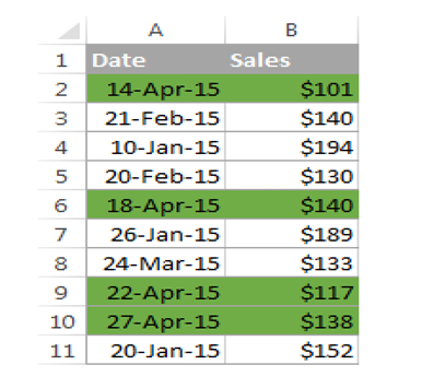
From the last instance in the table, if you intend to highlight all the rows with the present date of the month
First of all, you bring out the number of the month from dates in column A using the simplest =MONTH ($A2) formula. And then, you compare those numbers with the current month returned by =MONTH (TODAY()). As a result, you have the following formula, which returns TRUE if the months' numbers match, FALSE otherwise:
=MONTH($A2)=MONTH(TODAY())
Invent a conditional formatting rule in the Worksheet using this formula, and your outcome will look like these screenshots below (All the dates in April are highlighted as the write-up was prepared in April).
Highlighting dates within the current month
Example 2. Highlighting dates by month and day
Another difficulty you might encounter is wanting to highlight holidays while using this function, e.g., Xmas and New Year's days. How will you go about it?
In order to obtain a month's day (1-31), you can easily use the DAY function in Excel and use the MONTH function to obtain the number of a month. After this, confirm if the DAY is equivalent to 25 or 31, and also whether the month is equivalent to 12:
=AND(OR(DAY($A2)=25, DAY($A2)=31), MONTH(A2)=12)
Highlighting dates by month and day
The MONTH function operates in this manner in Excel. From all indications, it is obvious that it has a lot more uses than we have thought of before, right?
A SUMIF formula to sum data by month in Excel
If you don't want to attach an assistant column to your Worksheet, you are free to let it go. You can work a treat using the SUMPrODUCT function:
If you'd rather not add a helper column to your Excel sheet, no problem, you can do without it. A bit trickier SUMPRODUCT function will work a treat:
=SUMPRODUCT((MONTH($A$2:$A$15)=$E2) * ($B$2:$B$15))
Where column A contains dates, column B contains the values to sum, and E2 is the month number.
Note. The solutions above sum up all the values for a given month, paying less attention to the year, i.e., no specified year. Thus all of the values will be added up if your Worksheet embeds data for so many years.

In our upcoming write-ups, we are going to show you more tricks by giving you workouts for weeks and years. You can go through our previous Dates series in Excel (the links are below) if smaller time units interests you. I'm very grateful to you all for finding time to go through these tutorials until we bring you more tutorials next week!