Data can be complex and simple depending on the tasks performed on them. There are cases where we compare data between large groups. In such cases, it becomes tiresome to compare the data because the workload becomes more and more. After all, it becomes hard when the data starts dividing even more and more into smaller sub-groups from the main large group. In such cases, excel helps in solving such issues.
Excel through the function VLOOKUP enables completion of such tasks enabling the completion of such tasks in an accurate, fast, and effective way. For example when one is told to find a town in a recorded database. This can be done by assigning the task to excel where the data is combined and the place becomes easier to find.
One takes the different countries and the different results become displayed hence finding the place in the database. This task is a bit complex because the data must have been recorded accurately. It is completed by the use of other helper columns where the data is displayed. The helper columns are where the data reflects upon.
Step 1
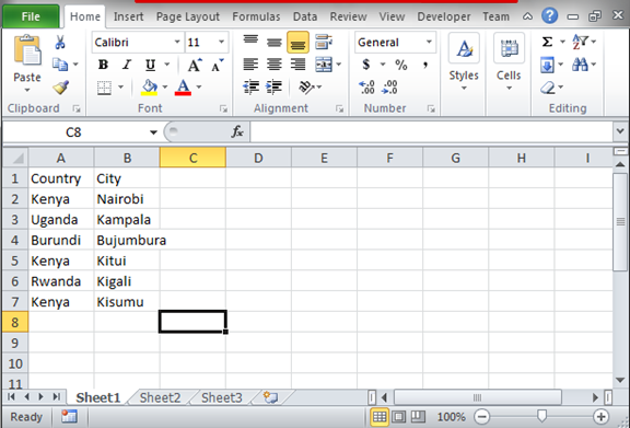
From your computer, open the excel sheet where you have the data records to work on. Below is a sample of such an excel sheet record.
Step 2
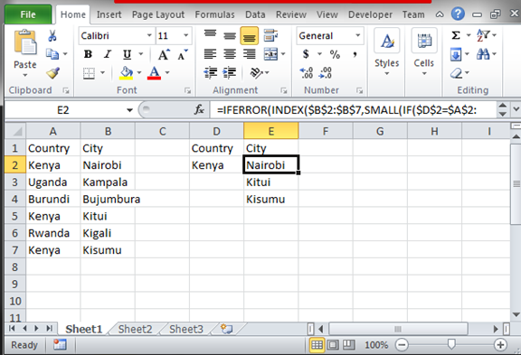
In this step, we will get the corresponding values vertically in the above data set. To get the values, write the formula below in the formula bar. =IFERROR (INDEX ($B$2:$B$7, SMALL (IF ($D$2=$A$2:$A$7, ROW ($A$2:$A$7)-ROW ($A$2) +1), ROW (1:1))),""). In the formula, B2: B7 is the column with the values that we want to return. A2: A7 is the column with the criteria and D2 is the column with the specific criteria where the values are displayed vertically in column E.