What is transpose function?
Transpose function is a function used in excel to convert a vertical range of cells to horizontal or convert the horizontal range of cells to a vertical range of cells. What the transpose function does is flip the orientation of the cells.
The first row becomes the first column, the second row becomes the second, and the third row becomes the third column of the new array when the array is transposed.
Transpose is used in both ranges and arrays. The ranges that are transposed are dynamic.
Paste special transpose
Paste special transpose is used as an option to switch columns to rows or rows to columns in excel. Alternatively, you can use the transpose function.
How to use Paste Special Transpose
To transpose data using paste special transpose the following steps are followed;
1. Select the range of cells that you intend to transpose; For example A1:C1
2. Right-click on the selected range then click copy.
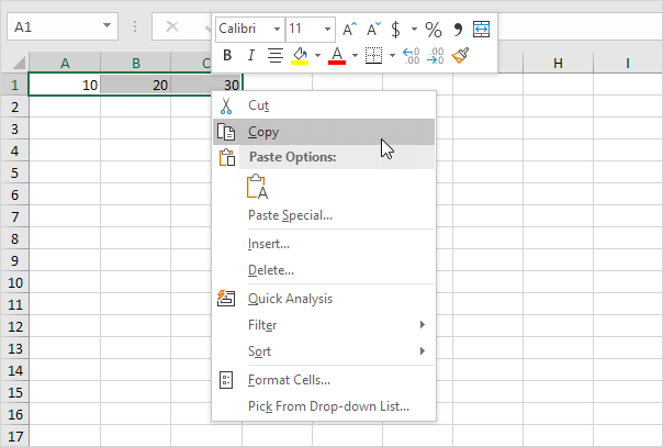
3. Select where you are going to paste in our case E2.
4. Right-click and then paste on then paste Special.
5. Check on the box of paste transpose and click ok.
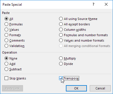
6. This would appear as shown below;

The use of Transpose Function
To insert and use the transpose function, follow the steps below;
1. Firstly, select the range of cells to be transposed.

2. Using the transpose function =TRANSPOSE (and select the range A1:C1 and close with a parenthesis)

4. When you are done finish by pressing CTRL + SHIFT + ENTER.

By wrapping it in curly brackets, the formula bar shows that this is an array formula. Select the range E2:E4 and hit remove to delete this array formula.
Transposing tables without zero
By using the transpose function in excel blank cells are converted to zeros, the IF function is simply used to solve this problem.
1. An example is cell B4 which is blank. This blank cell when transposed is converted to zero.

2. If the cell is blank, the IF function returns an empty string to transpose. A double quote with nothing in between.

Using the paste special transpose option is a good way to transpose but you may desire to link the source cell to the target cell. This can be achieved by just a few magic tricks.
1. Select the range of cells that you want to transpose A1:E2.
2. On the selected range, right-click and then click copy.
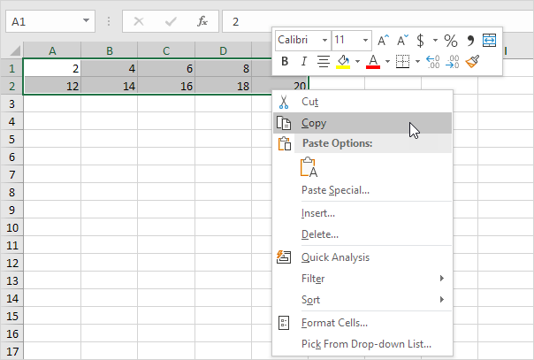
3. Select the desired point where you want to paste. A4
4. Next, Right-click then on "paste", select paste special.
5. A Paste special window will pop up. Click Paste Link.
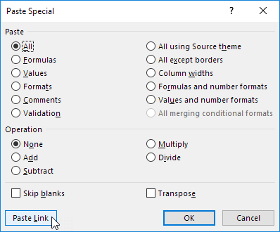
Result.

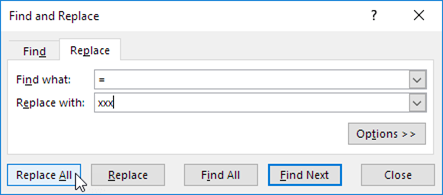
6. Choose the range A4:E5 and replace all the equal signs with xxx.
Result.

7. Using the paste special transpose method transpose the data

8. Select the range G1:H5 and replace all occurrences of 'xxx' with an equal sign giving an opposite of what was done on step 6.

You will notice that a link will be formed from the original cells to the transposed and once any change is made on the original range the transpose also changes.
In conclusion, when you intend to alter data by flip-flopping, you need not do it manually. Excel transpose will be handy and a faster way to solve the task.
