
When you are dealing with large excel worksheets that have a lot of rows and columns, in default, the heading will be unviewed when you scroll down your worksheet. Sometimes, you may want to make the header row freeze so that you can keep on referring to the headings without getting confused. Here, we give you different tips on how to keep your excel heading locked in place when scrolling through data in your worksheet.
Why do we lock worksheets cells, rows, or columns?
The most benefit you get when locking or freezing rows, columns, and cells is you get to see your important information regardless of scrolling the worksheet. The locked row always stays fixed making it easier to keep track of the column or rows identifiers. It also helps one avoid losing focus and entering data in the wrong cells.
Using the Freeze Panes function in Excel to freeze the top row
1. On your computer, access your Microsoft Excel Program.
2. Shift to the worksheet that you need to make your header freeze.
3. On your heading row, select the first cell.
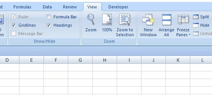
4. Go to the View tab on the main menu.

5. Click on the drop-down arrow under the Freeze Panes option.
6. On the drop-down list, click on the option Freeze Top Row. Now, your heading row will be frozen. You will be able to see it when you scroll down your data.

Note;
A frozen or fixed heading row will have a darker horizontal line underneath the first row.
You can also use some keyboard shortcuts to lock in your heading row. To do this, press Alt + w + f + r
Freezing or locking the first column in excel
At times a heading might be in a certain column or different columns. To lock the header in place, here is what to do;
1. First, open your excel worksheet.
2. Next, click on the View tab on the main menu ribbon.
3. Click on the drop-down arrow on the Freeze Panes option. It is a small triangle in the lower right corner.
4. On the drop-down list, click on the option Freeze First Column. To see whether your command has worked, scroll across your worksheet. Your left most column should stay fixed.
Apart from using the excel inbuilt function, you can freeze them first column by using the keyboard shortcut; Alt + w + r + c
Steps on how to lock top row and first column in excel
1. On your computer, open your excel spreadsheet.
2. Click on the first cell after your header row and column. It will be the column that is in the upper-left corner of the range that you want to remain locked. For example, if row 1 represents is the heading row, and column A has different headers, click on cell B2.
3. On the main menu, click on the View tab.
4. On the Freeze Panes, option, click on the drop-down arrow to display a drop-down list.
5. Select the option Freeze Panes. Doing this should freeze both your first row and first column.

You can also use the keyboard function Alt + w + f + f. all you have to do is make sure that you clicked a cell first.