A pivot table is a table that is used to summarize your table into an easily understood table. To a new Excel user, creating a pivot table from your data may be challenging. Don't worry, because this article got you covered. We shall discuss how to create a pivot table from the scratch using simple steps.
1. Enter your Dataset
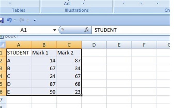
A pivot table is created the same way an Excel table is created. Therefore, you need to enter your data in rows and columns.
Your table should have headers also.
2. Insert Pivot table
Once all your data is set, you can now proceed and create a pivot table.
- Firstly, click on any cell on your dataset.
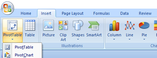
- On your main screen, locate and click on the "Insert" tab.
- On the left side, there is a section named Tables. From this section, click the pivot table drop-down button.
- From the drop-down menu, choose "Pivot table" since we are creating a pivot table. Click on it.
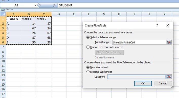
- A Create pivot table dialogue opens. This is where we add the Pivot table detail.
- Highlight all the columns and rows you want to summarize.
- Toggle on the"New worksheet" button.
- Finally, click the "Ok" button.
3. Dragging Fields
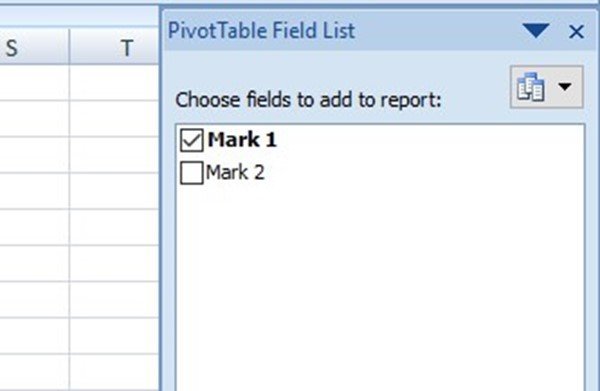
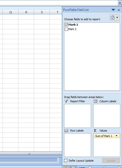
After clicking the "Ok" button on the Create Pivot table dialogue box, a PivotTable field pane opens on the rightmost side of the screen.
You can use this Field Pane to summarize your table.
Steps to do so;
- To show the result of each column in your PivotTable, simply check the checkbox next to the name of that column.
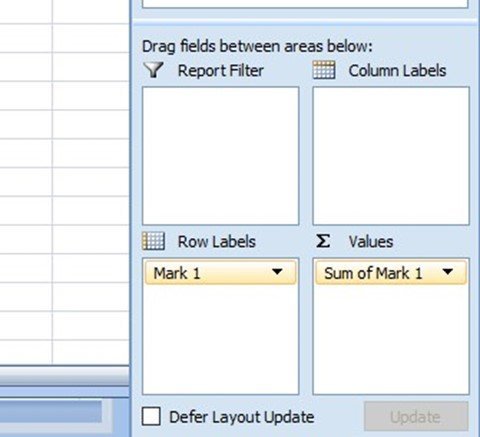
- Also, you can summarize by dragging the rows in your Pivot Table into the Field panes below.
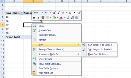
4. Sort
During statistical analysis, sorting is a vital practice. Here are the steps to sort your data in a PivotTable.
- Select any row by dragging it to the Row Labels section.
- Click any cell, within thin the displayed column.
- Then, right-click and click on the "Sort" button.
- From the sort side view menu, select the sorting type you want to apply to your data and click on it.
5. Filter
With the Excel PivotTable feature, you can filter the data on the table and extract a certain portion of information.
Here are the steps to do so;
- Drag the column you want to filter data from into the "Report field section."
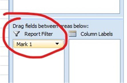
- The data from the row selected will appear on the main screen.
- Go ahead and click on the drop-down button next to the name of the column you had in the "Report field section."
- Using the checkbox, select the rows you may wish to filter.
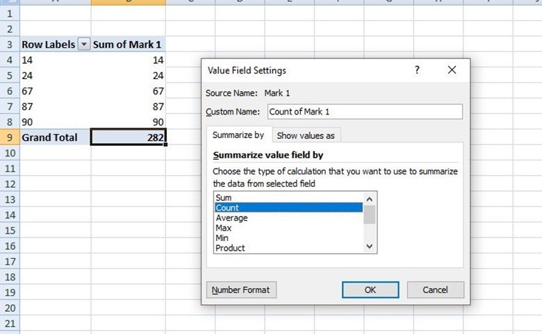
6.Changing summary calculation
Here are the steps to Change summary calculation;
- Click on any cell within the Sum Of amount column, and then right-click.
- From the side-view menu, choose the "Value field setting."
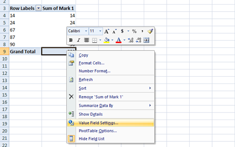
- In the dialogue box, choose the type of calculation you want.