Day to day records is being set, stored, and maybe forgotten. Every day institutions bring out different records whether they are on the expenditure of the institution or the normal running of the institutions. This ensures that people need to work hard to set the records straight. For example in a firm of over 500 workers and u want to know the number of people that are earning an amount higher or lower than a certain limit minding that the data is on different columns because of the different departments in the firm.
The only simple way to solve such a case is to highlight the colors of the cells. For example, for people who earn higher than that amount their cells are green while the others have a blue cell. This trims down the number of people from a very large group to a smaller identifiable and traceable amount of people.
The cells are advantageous in that they change colors depending on the value that is in the cells. In a case where the value moves higher or lower than the limit surpassing its initial value then the cell automatically changes. This ensures the data is accurate even if changes occur.
Step 1
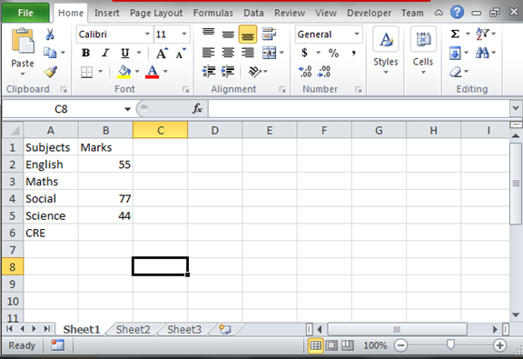
Open a blank excel sheet from your computer and record some data into it. If you have any existing record, feel free to use it. An example is the one below.
6
Step 2
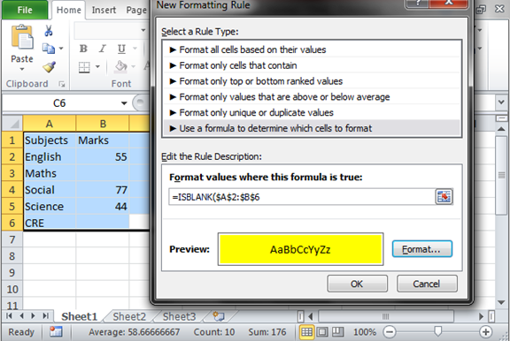
From the above data, we need to color the blank cells or change from the original color to a different color. To so, highlight the entire data set to start making the changes. Under the Home tab, select the conditional formatting option to reveal the list of other options. Select the new rule option at the bottom. A new window of options will appear shortly. Choose the option; use a formula to determine the cells to format. Insert the range of values you want to be formatted in the text box format the values where the formula is true. Now click on the format to set the color you want to use on the rows

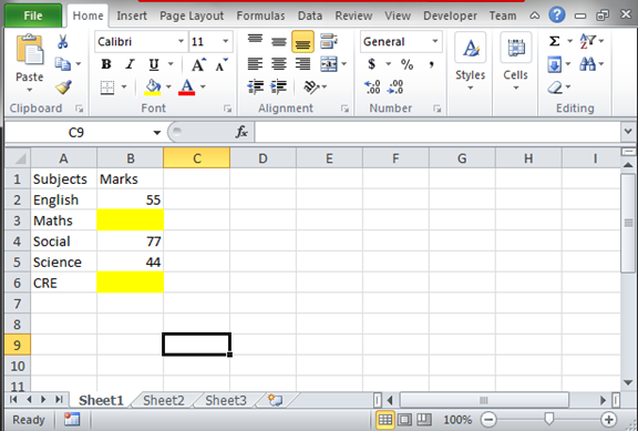
The formula will color the blank cells in the selected range.

