
There are a couple of ways to represent data in the excel sheets. You can use the rows and columns; you can use the tables and also the graphs. We represent data to make it more visible and clear to interpret. One of the tables used is the pivot table. A pivot table is just a statistical table that summarizes data in a more meaningful way. It explores and summarizes large amounts of data.
The data recorded in the pivot tables can contain dates or events that require dates. When we come across such data, we need to sort the data in the pivot table. To sort the dates we can arrange them in a certain order. For example, we can sort dates from the newest to the oldest and vice-versa. The following steps can be followed to sort the dates in a pivot table.
Step 1
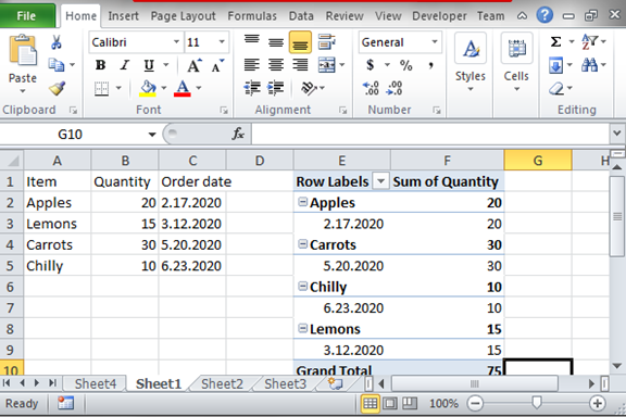
For us to sort the dates, we need to have the pivot table in place. To create a pivot table, insert some data in the rows and columns, and remember to have dates in them. Select the entire inserted data set and click on the insert menu. Under the Insert menu choose the pivot table, assign it the location and click on the ok button to finish. Consider the pivot table below.
Step 2
From the above pivot table, we have created, we can sort the dates in any order we would like to. The pivot table displays data in a more summarized way and the values appear as a summary. It is hard to pull out a single value from the pivot table. For us to sort the dates, we are going to only make the date's column visible. We do this by unchecking the items and quantity checkbox on the right of the sheet. Now with our date column, we can sort the dates. Highlight the dates without the column header and click on sort and filter located at the far right of the Home tab. Choose the options sort from Z to A. The dates will be sorted from the newest to the oldest. After sorting the dates, you can now check the other columns to have the pivot table visible as a whole.
