Rows in the excel sheet hold information in lines moving from the left of the sheet to the right of the sheet. The information in the rows can be related in one way or the other. By the physical appearance, you can tell what a certain row contains without having to be keen. In cases where you want to get the data clearly, you can choose to shade the rows to stress on. Shading is just the addition of background color in a row to make it distinct from the others.
A shaded row is visible and tells the view more about it. It can tell the viewer that it about its importance and so it should be considered. Shading does not mean that the row is more crucial than the others; sometimes we shade to filter the rows out from the others. We can shade the rows to count them or even delete them. We can use certain criteria to ensure that the second or the top row can always be shaded. This brings uniqueness to the excel sheet. The steps involved when shading the second row are as follows.
Step 1
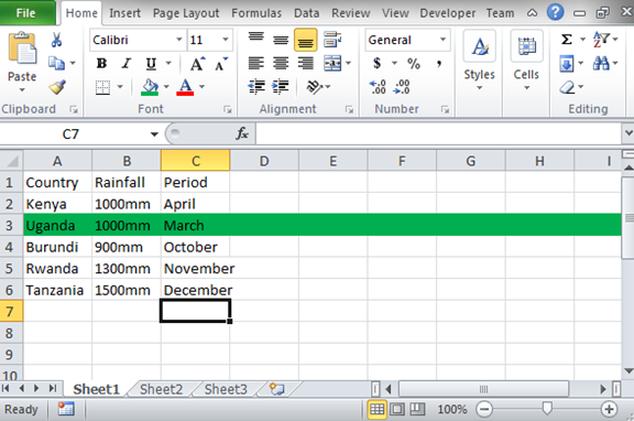
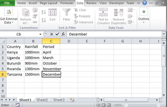
Open a blank excel sheet and record data in the rows if you do not have existing excel records to use. You can use the sample example below.
Step 2
For us to shade every second row, we need to set a new rule. The rule will help us to always shade every second row in the excel sheets. To set the new rule, select the entire data record. On the Home menu, select on conditional formatting under the styles group. Click on the new rule option under conditional formatting. In the window that appears, choose to use the formula to determine which cells to format and insert the formula =MOD (ROW (), 2) =0 in the textbox below. Click on the format option to enter the color you want to use while shading and click ok.