Excel uses tables to display and present data of certain findings. Tables present data in rows and columns but make it more clear and visible to interpret. The data to be displayed in the table is first in the form of excel rows and columns that is the default mode in all excel sheets. The data will then be displayed in a table form once you execute the table command. To view data in a table you select the entire data and insert a table from the Insert menu.
The process of inserting the table and having your data displayed in the table is what we refer to as format as a table. The data will be formatted in the form of a table. To cancel the format as a table, you go back to the original data range you had before inserting a table. The following steps can guide us on how to remove the table formatting.
Step 1
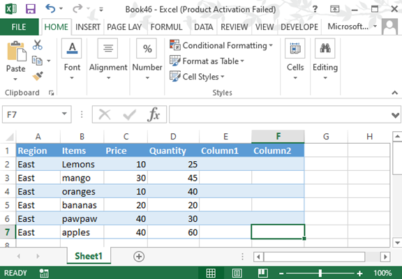
To remove the table formatting, open the excel sheet where you have inserted the table. In case you do not have the table, you can create some data range and format it into a table to make sure you get the concept of removing the table format. We need first to format the data into a table to make the process of removing the formatting effective. Consider the sample below.
Step 2
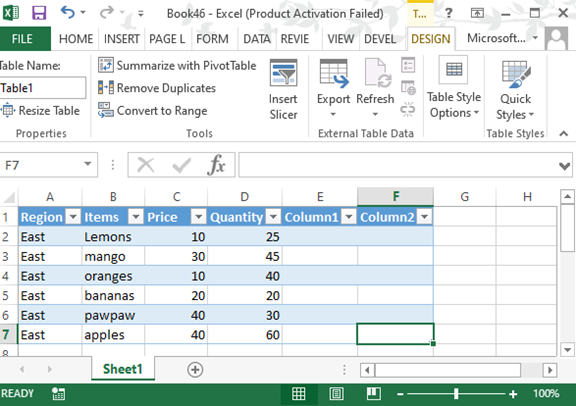
The above data set has been formatted into a table. To get back to the original data set, we need to remove the table formatting. To remove the table formatting, go to the design menu and under the tools section, click on convert to range option. A popup window appears shortly asking you whether you want to convert to the range. Click on the ok button and your data will be converted to the range. With that, the table formatting has been removed.