When working with an excel worksheet that contains large data sets, you may need to keep your top rows visible. Most times, users do this to keep track of what they are working on and to avoid making entry mistakes on what they are working on. It also makes it easier for someone to keep on referring to the data within their worksheet. Luckily, Excel has several tools that make it easier for its users to view the top row or column from different parts within their workbook.
Here, we guide you on how to keep the top rows in excel visible. We also give you the different steps of keeping your columns visible.
Steps on how to freeze the top row or top column in excel
1. On your computer, open the Excel worksheet you want to freeze the top row.
2. On the main menu ribbon, click on the View tab.

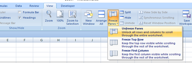
3. Under the Windows group, click on the Freeze Panes drop-down arrow.
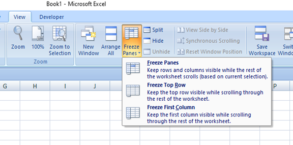
4. In the drop-down list, select Freeze Top Row.
5. Afterward, check your worksheet by scrolling up and down to see whether the top row will still be visible. To know whether it worked, Excel will automatically insert a noticeable thin line to show where the frozen pane begins.
But, what if you need to freeze several top rows within your worksheet. Here is what to do;
1. On your computer, open the excel worksheet.
2. In your worksheet, select the row that is immediately beneath the last row you want to freeze.
3. Click on the View tab on the main menu.
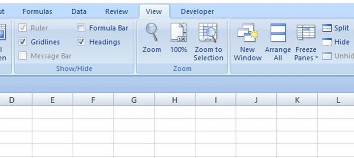
4. Under the Windows group, click on the Freeze Panes drop-down arrow.
5. Next, select the Freeze Panes option. Afterward, you will see that your multiple rows are still visible when you scroll through your worksheet.
Note;
Under the Freeze Pane drop-down list, you will come across different options. Here, you can also select 'Freeze First Column,' which will freeze or keep the leftmost column in your worksheet visible when you scroll through it horizontally.
How to get quick access to the freeze panes option
Any excel user can add a freeze button to the Quick Access Toolbar that would enable them to freeze the first column, top row, cells, columns, and cells with a single mouse click. Here is what to do;
- In your open excel workbook, click on the down arrow. The arrow is on top of the main menu ribbon where the undo and autosave options are.
- Click on the More Commands option.
- Under Choose commands from section, select the option Commands Not in the Ribbon.
- Select Freeze Panes and click Add.
- Click OK.
- When you want to freeze the top row, you will select the row you want to freeze and click on the magic Freeze button on the Quick access menu.
Steps to follow to unfreeze top row
1. In your open excel worksheet, go to the main menu ribbon.
2. Click on the View tab.
3. Under the Windows group, select the option Unfreeze Panes. After clicking on this option, you will notice that when scrolling through your worksheet, the row will not be visible.