It is possible to hide rows based on the cell value in columns and they will not be visible in your work depending on the criteria you choose to apply, either great then, small then, or even equal to respectively. For instance, you can choose to hide rows with a cell value below 100, like in our case in the work discussed below to help with your understanding. This is an example criterion with a made figure from a personal data set. The steps are as follows
We can choose to use the filter method to hide the rows based on the cell value as shown in the case below.
1. Select the data in the column you want to filter or hide it data, and click on the Data in the ribbon of your excel worksheet, and select filter.
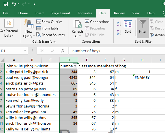
2. After you have selected the data for the filter, click on the filter down arrow in the column selected (the column you are working on, on the top left) to display the filter drop-down menu, then click on the number filter (or text filter irrespectively) and then click on greater than in the sub-menu. You can choose any other criteria you want to use depending on what you want to achieve.

3. Text the criteria you want to use in the drop-down pop-up menu in the greater than sub-menu as shown below. In our case, as earlier explained we are using greater than 100.

4. click ok. Now all the data in the cells with less than a 100 are hidden in the selected column and the cells will display any figure above a 100 as shown below.

With this formula you can only filter a column at a time one by one.