It is important to note that it is only possible to freeze top rows and columns of an excel worksheet from the top left, one cannot freeze rows and columns from the middle of a worksheet. Freezing rows and columns make the area visible as one scrolls down or to another area of a worksheet. Below are steps on how o freezes the top rows and columns in a worksheet.
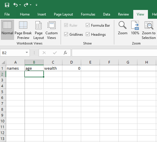
1. Go to the View bar in the ribbon of the worksheet and click on the freeze panes.

It is important to note that you can only freeze rows and columns simultaneously, if a row is frozen and you choose to freeze the column next to it the column will be frozen but the row will unfreeze. Additionally, it is important to note that the freeze panes will not be available when you are on cell editing mode or when the worksheet is protected. Press enter or esc to cancel editing mode.
2. Click on the freeze panes on the freeze panes submenu with your active cell on B2 and now the top row and column are frozen with a solid line showing on their bonders to indicate that they are frozen as shown below.
Note that you cannot freeze rows and columns and split them at the same time. Also if you want to freeze rows you should select a row below the rows you want to freeze and click on the freeze panes freeze rows on the view of the ribbon, same case applies when freezing columns, you select a column next to the columns you want to freeze and click on the freeze columns on the freeze panes of the view bar of your excel worksheet.